Using RL to maximize ad revenue without retention tradeoffs
Using Contextual Bandits and Predictive Modeling to Optimize Personalized Ad-Placement Policies


Global Ad industry hits $1 trillion in revenue. In this blog, we will learn how to maximize ad revenue with minimal impact to retention and engagement.
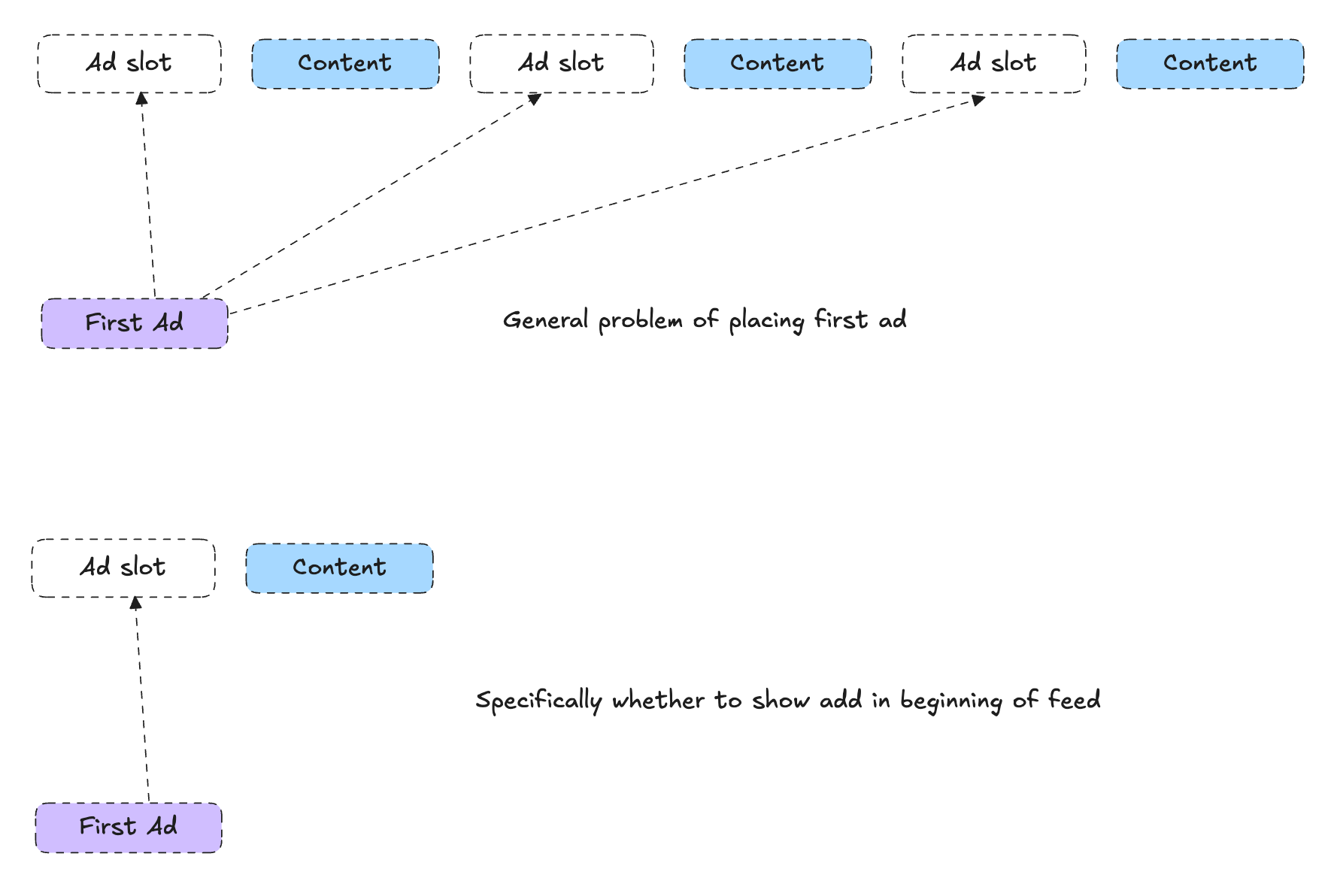
In a content platform like YouTube, deciding whether to show an ad as the very first piece of content is a subtle but critical problem. The trade-off is intuitive:
If you show an ad first: You gain immediate ad revenue, but you risk users dropping off or engaging less with the subsequent content.
If you don’t show an ad first: You keep the user more engaged (likely increasing future content consumption and potentially downstream revenue), but you sacrifice the immediate revenue opportunity of that first impression.
In this post, we’ll explore how to frame this decision using a data-driven approach. We’ll start from a simplified viewpoint—just deciding whether to show an ad first—and build up to a strategy that integrates both engagement-based revenue modeling and personalized ad revenue predictions. We’ll then discuss how a contextual bandit approach can be applied to learn these policies from historical data.
#1: Blending Approach —> Engagement Loss improvement
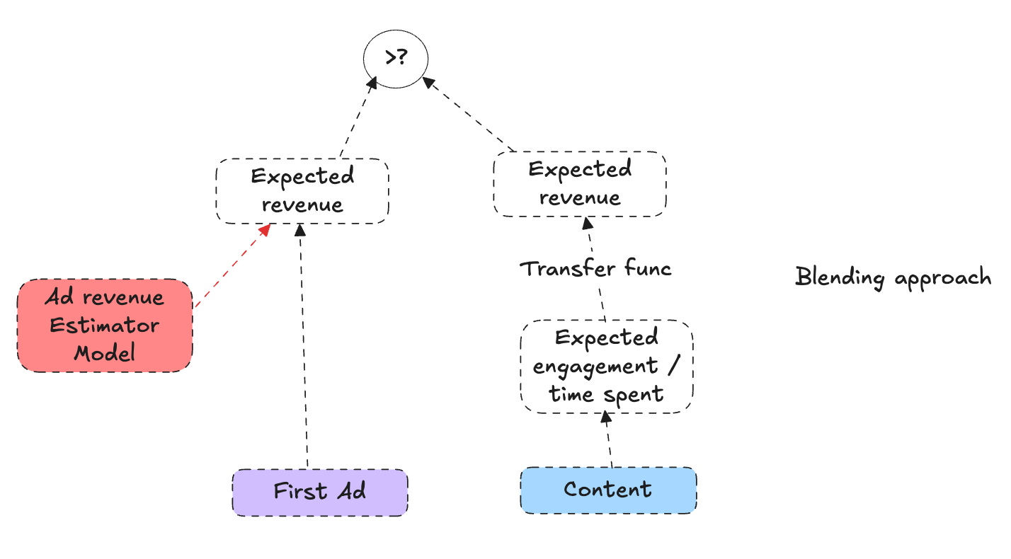
A first, naive approach might consider the expected revenue from showing an ad in the first position versus the expected long-term engagement if we skip that ad. We could imagine we have two signals:
Expected Ad Revenue (E[rev|u, ad]): A personalized model that, given the user and session context, estimates the immediate revenue we would earn by showing an ad. This might be well-approximated by an advanced personalized ads model trained on historical ad-serving data.
Expected Engagement: A measure or score indicating how much content consumption (views, watch time, etc.) we expect if we place content first. We assume we already have a way to translate engagement into revenue via a function
f_eng_to_rev(engagement), which converts user engagement into an expected revenue value (for example, predicting future watch-time-based monetization).
In a simple scenario, if we had some expected engagement value for showing content and some expected engagement value for not showing content, we might attempt to “blend” them with the direct ad revenue to decide. However, it’s not straightforward: the presence of an initial ad does not necessarily mean all engagement is lost—it just might reduce it. What we really need is the expected reduction in engagement caused by showing the ad.
For example, if for some deeply satisfied users their engagement will be mostly unaffected by showing the ad, it should be fine to show the ad.
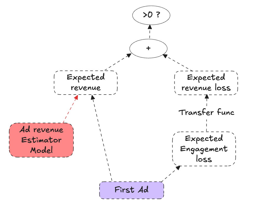
Let’s say we have estimated the expected engagement loss if we show the ad first. Our decision rule could look like this:
Show Ad if and only if: (engagement_revenue_conversion * expected engagement loss) < (expected revenue of showing an ad)
or mathematically
This equation says: “If the immediate ad revenue gain from showing the ad exceeds the revenue-equivalent cost of reduced engagement, then show the ad.” It relies on three components that can be learned independently:
E[rev|u, ad]: The expected incremental ad revenue from showing the ad first for a given user/session.
f_eng_to_rev: The function that converts changes in engagement into revenue terms.
Expected engagement loss: Learned from data, comparing engagement outcomes between sessions where an ad was shown first and sessions where it was not.
#2 Bridging Theory and Practice: Two Approaches in Our GitHub Repository
In our GitHub repository, https://github.com/gauravchak/ad-placement-rl, we demonstrate two different approaches to optimizing session revenue directly: a contextual bandit method and a reinforcement learning (policy gradient) method. In both cases, the setup is the same: at each session (context), we must make a binary decision—whether or not to show an ad—and we then observe a numerical reward. This reward is a combined metric that integrates both immediate session-level revenue and the engagement-based revenue equivalent.
Notably, these approaches can benefit from additional features in the user context. For example, even before we integrate the personalized ad estimator’s output (E[rev|u, ad]) into the reward function, we can include it as part of user_features. By doing so, both the contextual bandit and the policy gradient models can leverage this personalized signal at inference time, potentially improving decision-making and anticipating the value of showing an ad first.
Building steerability in net reward
There might be times in the year, like say thanksgiving, when your business wants to prioritize revenue. It might help to build a dial for that.
2a: Optimizing session net reward Contextual Bandits
Code Snippet on whether to show ad:
def should_show_ad(reward_model_ad, reward_model_no_ad, user_features):
    """
    Given trained reward models and user_features, return a decision:
    show_ad = 1 if predicted_reward_if_ad > predicted_reward_if_no_ad else 0
    """
    pred_net_reward_if_ad, pred_net_reward_if_no_ad = expected_reward(
        reward_model_ad=reward_model_ad,
        reward_model_no_ad=reward_model_no_ad,
        user_features=user_features)

    # True if predicted net reward of ad action is higher
    return (pred_net_reward_if_ad > pred_net_reward_if_no_ad)
This contextual bandit approach trains separate models to predict the expected reward under each action. By comparing these predictions, the policy picks the action that yields the higher expected combined value at inference time. It’s conceptually simple and can be effectively trained on logged data, making it a practical first step toward data-driven ad placement decisions.
2b REINFORCE and Policy Gradients
While contextual bandits are a simple and effective way to learn a policy directly from logged data, they still treat each decision as a one-step problem. Another approach, inspired by reinforcement learning (RL), is to use policy gradient methods such as REINFORCE.
A great tutorial of using Deep RL for a binary decision is Andrej’s talk below on Pong
Conceptual Overview
In the REINFORCE framework, rather than training separate models to predict the reward for each action and then comparing them, you directly parameterize a probabilistic policy that decides how likely it is to show an ad or not. For each training example, you know which action was taken and what the resulting reward was. The goal is to adjust the policy parameters to increase the probability of actions that led to higher rewards and decrease the probability of actions that led to lower rewards.
By doing this, REINFORCE naturally fits the problem of deciding whether to show an ad first: you have a distribution over actions, and you tune it to favor whichever action yields better long-term value. If showing ads first consistently produces higher combined revenue (ad revenue plus engagement-based returns), the policy naturally shifts towards showing the ad. If it reduces future engagement too much, the policy learns to refrain from showing the ad.
Why REINFORCE?
Direct Optimization: REINFORCE directly optimizes the expected reward of the policy. Instead of separately learning a model for each action and then deriving a policy, you adjust the policy parameters to maximize the observed rewards.
Built-in Exploration:
By modeling a probability distribution over actions (instead of choosing actions deterministically), the policy naturally explores different decisions. This stochasticity can help the algorithm discover better policies that might be missed by purely greedy strategies. By outputting probabilities over actions, the policy gradient approach allows you to sample actions according to those probabilities, rather than always taking the single top-scoring action. This means the model inherently tries different actions over time, which can lead to discovering better strategies than a purely greedy (deterministic) approach would.Generalization to RL Settings: Although we’re currently working in a single-step contextual bandit setting, policy gradient methods can easily generalize to multi-step reinforcement learning problems. This opens the door to modeling scenarios where the consequences of showing (or not showing) an ad extend beyond the first position, or even the current session.
Pros and Cons of REINFORCE vs. Contextual Bandits
Pros (REINFORCE):
Directly learns a stochastic policy that can be generalized to more complex sequential or multi-step decision-making scenarios.
Conceptually simple: the update rule is just scaling the log probability of the chosen action by the reward.
Cons (REINFORCE):
High variance: The basic REINFORCE update can be noisy and may require techniques like baselines or variance reduction to stabilize training.
On-policy: The method is conceptually on-policy, meaning it learns best when data is collected from its own evolving policy. Using strictly logged offline data (collected by a different policy) can introduce bias unless steps are taken to correct it.
Pros (Contextual Bandits):
Simpler, more direct learning: Estimate the reward for each action and pick the best one. Straightforward modeling from logged data.
Lower variance estimates: Predictive models for each action can produce more stable estimates with offline data.
Cons (Contextual Bandits):
Limited to single-step decisions: The approach doesn’t naturally extend to sequential decision-making.
Requires a separate model for each action or a common model architecture that outputs multiple action values.
#3 - Integrating the Ad Revenue Estimator (E[rev|u, ad]) deeply
In Part 2, we’ve discussed incorporating E[rev|u, ad] as an input feature. This is helpful, but we can push the idea further by explicitly decomposing the reward. Instead of lumping all revenue and engagement value into a single session label, we can separate the immediate revenue from showing an ad (predicted by E[rev|u, ad]) from the delayed, engagement-based revenue. In other words, we estimate:
Immediate Reward (if ad is shown):
E[rev|u, ad]—our personalized ad revenue estimate.Delayed Reward (if ad is shown): Session value minus the immediate ad revenue, converted into engagement-equivalent terms.
At inference time, this lets us approximate the decision boundary more explicitly. We compare the sum of the immediate and delayed rewards for showing the ad against the expected session value if we do not show the ad:
This approach leverages the fact that our immediate revenue estimates are likely of higher accuracy and reduces the complexity of what we must learn as a “residual” (delayed) effect. It ties together the personalized ad estimator with a session-level RL framework, enabling more accurate and modular policy decisions.
Summary
We show how to use RL to learn when to show an ad.
The framework extends to other positions, not just first position. The RL policy encapsulates exploration to enable continuously improvement.
We do so in a way that maximally uses our high accuracy ad revenue estimator model. Thus we have set up the problem in a modular fashion with multiple teams working in synergy.
Disclaimer: These are the personal opinions of the author(s). Any assumptions, opinions stated here are theirs and not representative of their current or any prior employer(s). Apart from publicly available information, any other information here is not claimed to refer to any company including ones the author(s) may have worked in or been associated with.
 | A guest post by
|
ML based Ad placement is a small community. We would love to hear from others in this community.