Sampling : the secret of how to train good embeddings

Machine learning solutions are the industrial state of the art in most search, recommendations, online ads, high frequency trading and self driving applications. Irrespective of the industry, a key ingredient in the quality of the model/embeddings is the data distribution that is used to train the model.
Sampling and auto-labeling of the sampled cases is basically where most of the work is happening in applied ML teams.
About half of the above CVPR 2021 talk by Andrej Karpathy, for instance, talks about sampling and auto-labeling of interesting cases to feed their vision-only perception model.
Outline
In this article we will look at evolution of sampling from a first principles approach. We will restrict ourselves to multi-class classification.
We will see why sampling is needed for efficient training of embeddings / classification models.
We will see a method, in-batch negatives, that is super fast but produces embeddings that lead to unpopular items.
We will see how to correct it via importance sampling.
We will bring it all together with Mixed Negative Sampling.
For those who want to skip to the “solution” and learn about what to implement in their model training pipeline, please jump to the “Mixed Negative Sampling” section below.
(If you want to discuss sampling approaches in other settings like high frequency trading and self driving, please follow up on email)
Probability of selection of an item
A common way to express the probability of outcome y (ad click if shown / search result click / object type recognized ) given input x (user / query / image) is
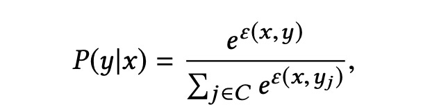
The formula above claims that if you give me an embedding of the input x then the probability of the output being y from a set C of options is proportional to the exponent of the dot product of the embedding of x and the embedding of y.
i.e. P(y|x) ∝ exp ( embedding (x) dot embedding (y) )
For instance, for a short video app like TikTok, y would be a video in your corpus, x would be the user features and user history.
Now to make something a probability, you need to have a summation over all possibilities in the denominator. It is easy to see that computing the denominator becomes computationally expensive when the set of possibilities C is large. However, before we solve that problem, let’s try to understand the effect of a large C in serving results and in training.
Serving is unaffected by the large corpus size
Serving of results refers to what needs to be done when a user request comes in.
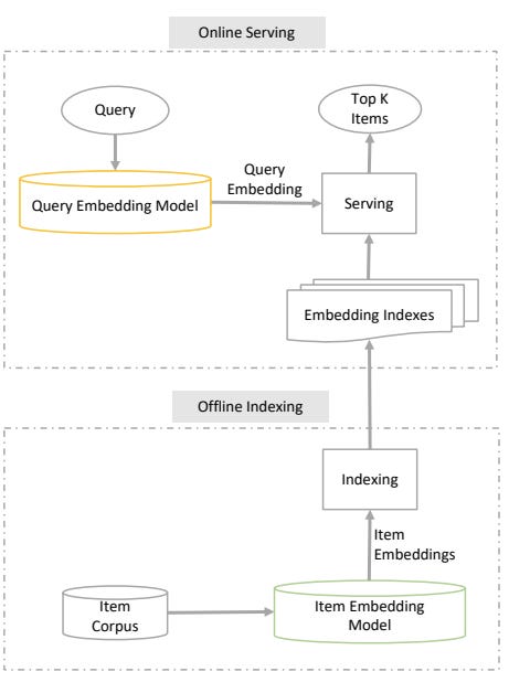
As shown in the above image, during the retrieval phase the set of possible items, C, could be in millions. However, since the denominator is the same for all items, this amounts to choosing the top-100 or so items by the dot product of query and item, i.e (embedding (x) dot embedding (y)). Since there are efficient solutions for Maximum Inner Product Search (like ScaNN), we don’t need to worry about the large C during retrieval.
Training of each example requires updating the entire corpus!
The problem does not go away during training time though. For each instance of a positive example {query, results clicked}, it seems like we need to compute (embedding (x) dot embedding (y)) with y ranging over the entire corpus. We also need to backpropagate and update the embeddings of each item. That means, for a corpus with 100 million items, we are doing 200 million operations per interaction that we are learning from.
Let’s ask ourselves what my algorithms course instructor Dr. Sanjeev Khanna kept asking students in every class … “Can we do better?”
Using Negative Sampling to avoid training on the entire corpus
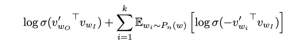
In Distributed Representations of Words and Phrases and their Compositionality (Mikolov et al. 2013), the authors try to solve this in the context of NLP and word vectors. They say that the denominator is in expectation equivalent to sampling a few negatives from the corpus and not using all of them.
In the video below, Dr. Andrew Ng has explained the same:
Using In-batch negatives to reduce training time
Mikolov et al. 2013 also introduce an optimization that is particularly useful for GPU based computation, that of in-batch negatives. If we take a batch of 1024 positive examples, {query, result}, then every result in the batch that is not the same as the one that was clicked for the query can be used as a negative.

This works well in practice. Training is fast due to the implicit compute parallelism of the GPU.
Use importance sampling to correct (un)popularity bias of in-batch sampling
However, the distribution of negatives is not what we were looking for in Fig 3 above. For instance, the in-batch negatives are all taken from items some other user has clicked. Hence they are more likely to be popular items.
To account for this, if an item selected has a distribution Q(y) in how the negatives have been sampled then Q(y) would have to be in the denominator. (Also referred to as Importance Sampling)
To understand why, suppose an item is sampled more frequently than uniform, then we should reduce the effect on the loss of every occurrence of the item. Remember that in Fig 1 at the top the denominator was a simple sum over all items in C.

Fig 5 above explains how the term for item j is exp(<u, v_j> - log(Q_j)) which is same as exp(<u, v_j>)/Q_j.
For a mathematically rigorous description of many approaches to sampling read this document on candidate sampling. It shows how to correct for the bias and how not correcting for the bias will train a function that is biased towards less popular items. (PS: These are a couple of threads that have tried to explain the candidate sampling document: negative sampling vs sampled softmax, on stackexchange)
A general application of importance sampling in Reinforcement learning based recommendations
In the famous REINFORCE recommender system paper, which shows a brilliant application of reinforcement learning to recommender systems, the authors address a similar problem. They have data from an existing sampling generator β and hence they need to divide the loss-gradient of the sample τ with β(τ).

Mixed Negative Sampling : An elegant simple solution to the above problems
We know the ideal solution for probability estimation is to sample uniformly.
We know that using in-batch negatives is very fast but produces a recommender that is biased against popular items.
Mixed negative sampling is an approach that basically does both, uses in-batch sampling and also uniformly sampled negatives.

A wonderful paper showing this works very well is Towards Personalized and Semantic Retrieval: An End-to-End Solution for E-commerce Search via Embedding Learning by JD.com search team.
Open question
Keen readers of Mixed Negative Sampling or Towards Personalized and Semantic Retrieval will note that both state that using items as “negatives” which where shown to the user but were not clicked by them leads to a worse outcome. The metrics regress. None of them really explain this empirical observation. What do you think? Why would that be the case?
Disclaimer: These are my personal opinions only. Any assumptions, opinions stated here are mine and not representative of my current or any prior employer(s).